球座標でデータをプロットする

緯度-経度座標のデータからメッシュを生成および表示します．

import numpy as np

import pyvista as pv


def _cell_bounds(points, bound_position=0.5):
    """
    Calculate coordinate cell boundaries.

    Parameters
    ----------
    points: numpy.ndarray
        One-dimensional array of uniformly spaced values of shape (M,).

    bound_position: bool, optional
        The desired position of the bounds relative to the position
        of the points.

    Returns
    -------
    bounds: numpy.ndarray
        Array of shape (M+1,)

    Examples
    --------
    >>> a = np.arange(-1, 2.5, 0.5)
    >>> a
    array([-1. , -0.5,  0. ,  0.5,  1. ,  1.5,  2. ])
    >>> cell_bounds(a)
    array([-1.25, -0.75, -0.25,  0.25,  0.75,  1.25,  1.75,  2.25])
    """
    if points.ndim != 1:
        raise ValueError("Only 1D points are allowed.")
    diffs = np.diff(points)
    delta = diffs[0] * bound_position
    bounds = np.concatenate([[points[0] - delta], points + delta])
    return bounds


# First, create some dummy data

# Approximate radius of the Earth
RADIUS = 6371.0

# Longitudes and latitudes
x = np.arange(0, 360, 5)
y = np.arange(-90, 91, 10)
y_polar = 90.0 - y  # grid_from_sph_coords() expects polar angle

xx, yy = np.meshgrid(x, y)


# x- and y-components of the wind vector
u_vec = np.cos(np.radians(xx))  # zonal
v_vec = np.sin(np.radians(yy))  # meridional

# Scalar data
scalar = u_vec**2 + v_vec**2

# Create arrays of grid cell boundaries, which have shape of (x.shape[0] + 1)
xx_bounds = _cell_bounds(x)
yy_bounds = _cell_bounds(y_polar)
# Vertical levels
# in this case a single level slightly above the surface of a sphere
levels = [RADIUS * 1.01]

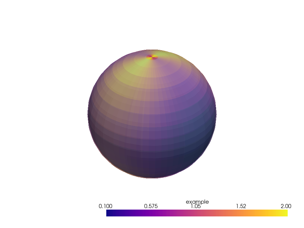
構造化グリッドの作成

grid_scalar = pv.grid_from_sph_coords(xx_bounds, yy_bounds, levels)

# And fill its cell arrays with the scalar data
grid_scalar.cell_data["example"] = np.array(scalar).swapaxes(-2, -1).ravel("C")

# Make a plot
p = pv.Plotter()
p.add_mesh(pv.Sphere(radius=RADIUS))
p.add_mesh(grid_scalar, clim=[0.1, 2.0], opacity=0.5, cmap="plasma")
p.show()

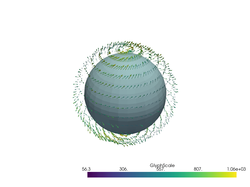
球座標でのベクトルの可視化垂直風

w_vec = np.random.rand(*u_vec.shape)

wind_level = [RADIUS * 1.2]

# Sequence of axis indices for transpose()
# (1, 0) for 2D arrays
# (2, 1, 0) for 3D arrays
inv_axes = [*range(u_vec.ndim)[::-1]]

# Transform vectors to cartesian coordinates
vectors = np.stack(
    [
        i.transpose(inv_axes).swapaxes(-2, -1).ravel("C")
        for i in pv.transform_vectors_sph_to_cart(
            x,
            y_polar,
            wind_level,
            u_vec.transpose(inv_axes),
            -v_vec.transpose(inv_axes),  # Minus sign because y-vector in polar coords is required
            w_vec.transpose(inv_axes),
        )
    ],
    axis=1,
)

# Scale vectors to make them visible
vectors *= RADIUS * 0.1

# Create a grid for the vectors
grid_winds = pv.grid_from_sph_coords(x, y_polar, wind_level)

# Add vectors to the grid
grid_winds.point_data["example"] = vectors

# Show the result
p = pv.Plotter()
p.add_mesh(pv.Sphere(radius=RADIUS))
p.add_mesh(grid_winds.glyph(orient="example", scale="example", tolerance=0.005))
p.show()

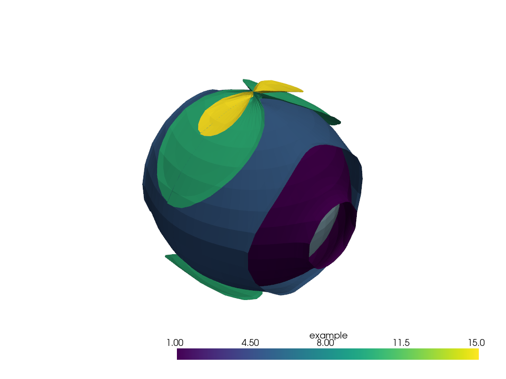
球座標の3 Dデータのサーフェス

# Number of vertical levels
nlev = 10

# Dummy 3D scalar data
scalar_3d = (
    scalar.repeat(nlev).reshape((*scalar.shape, nlev)) * np.arange(nlev)[np.newaxis, np.newaxis, :]
).transpose(2, 0, 1)


z_scale = 10
z_offset = RADIUS * 1.1

# Now it's not a single level but an array of levels
levels = z_scale * (np.arange(scalar_3d.shape[0] + 1)) ** 2 + z_offset

# Create a structured grid by transforming coordinates
grid_scalar_3d = pv.grid_from_sph_coords(xx_bounds, yy_bounds, levels)

# Add data to the grid
grid_scalar_3d.cell_data["example"] = np.array(scalar_3d).swapaxes(-2, -1).ravel("C")

# Create a set of isosurfaces
surfaces = grid_scalar_3d.cell_data_to_point_data().contour(isosurfaces=[1, 5, 10, 15])

# Show the result
p = pv.Plotter()
p.add_mesh(pv.Sphere(radius=RADIUS))
p.add_mesh(surfaces)
p.show()