点群のプロット

この例では，PyVistaを使って 'points' と 'points_gaussian' の両方のスタイルを使い，点群のプロットを行う方法を紹介します．

from __future__ import annotations

import numpy as np

import pyvista as pv
from pyvista import examples

プロット方法の比較

まず，サンプル点群を numpy.random.random() を使って作ってみましょう．

# Seed rng for reproducibility
rng = np.random.default_rng(seed=0)
points = rng.random((1000, 3))
points

array([[0.63696169, 0.26978671, 0.04097352],
       [0.01652764, 0.81327024, 0.91275558],
       [0.60663578, 0.72949656, 0.54362499],
       ...,
       [0.1027894 , 0.60866026, 0.43809722],
       [0.95205703, 0.12833537, 0.77821681],
       [0.02483448, 0.20765295, 0.30052863]])

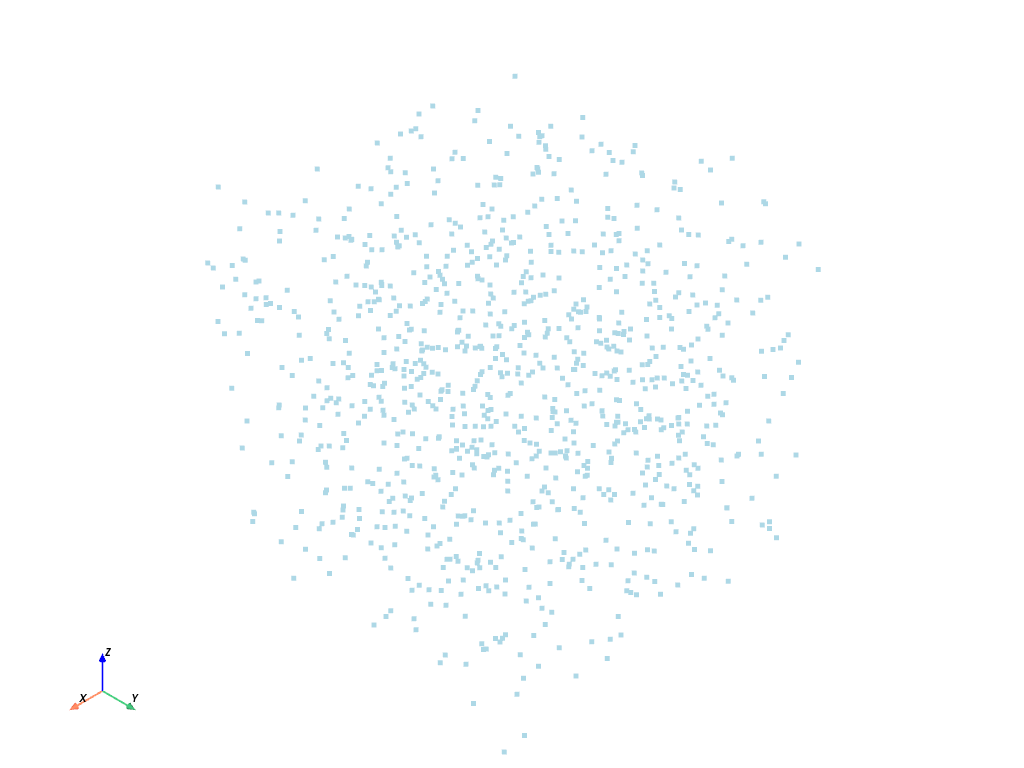
基本プロット

この点群は，便利な pyvista.plot() 関数を使って簡単にプロットすることができます．

pv.plot(points)

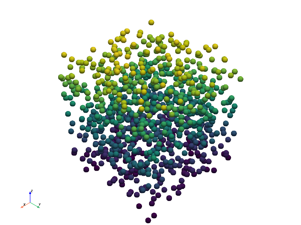
スカラーを使ったプロット

それではつまらないので，色をつけてみましょう．点をプロットするには，単一のスカラーを使うこともできます．例えば，z座標．

また，楽しみに，点を球体でレンダリングしてみましょう．

pv.plot(
    points,
    scalars=points[:, 2],
    render_points_as_spheres=True,
    point_size=20,
    show_scalar_bar=False,
)

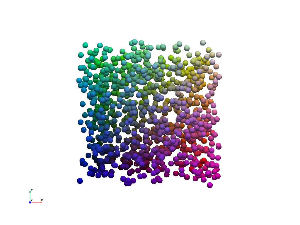
RGBAを使ったプロット

また，RGBA配列を使用して点群に色を付けることもできます．これは (0, 1) で正規化されていますが，0-255 の numpy.uint8 配列を使用することも可能です．

rgba = points - points.min(axis=0)
rgba /= rgba.max(axis=0)
pv.plot(points, scalars=rgba, render_points_as_spheres=True, point_size=20, cpos='xy', rgba=True)

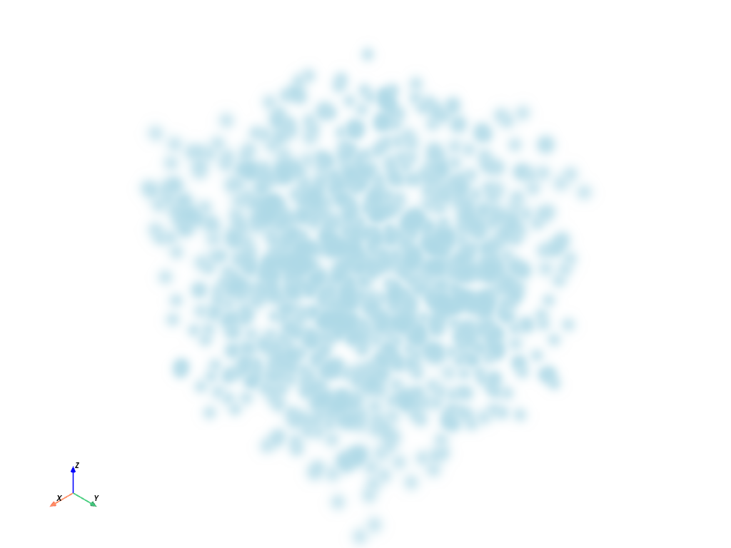
点群プロットスタイル

PyVista は 'points_gaussian' スタイルをサポートしており，点を個々のソフトスプライトとしてレンダリングします．また， render_points_as_spheres=True (デフォルト) を使用すると，レンダリングパフォーマンスを犠牲にして，よりソフトな点を作成することが可能になります．

再び基本的なプロットを示しますが，スタイルは 'points_gaussian' にしてあります．

pv.plot(points, style='points_gaussian', opacity=0.5, point_size=15)

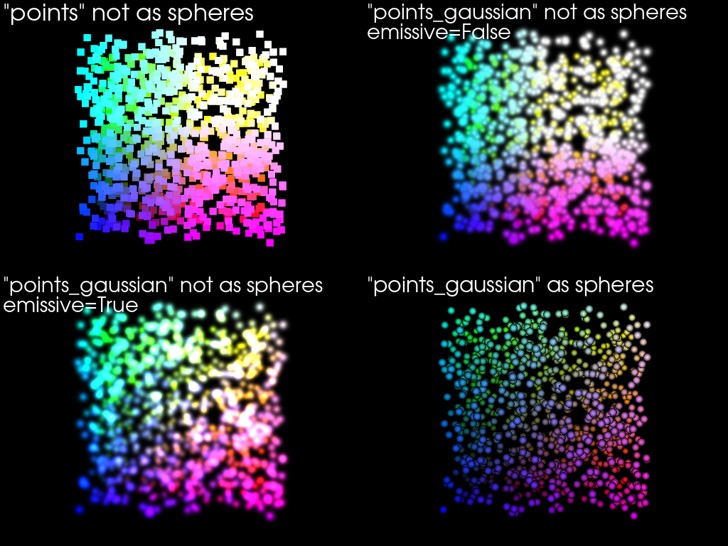
ここに，4つのオプションの組み合わせを並べたプロッタを示しますので，これらの点をプロットするときに利用できるさまざまなオプションを自分で確認することができます．PyVista は賢明なデフォルトを実現しようとしていますが，もしこれがあなたのニーズにとって不十分だと感じたら，遠慮なくいろいろなオプションで遊んで，あなたに合うものを見つけてください．

pl = pv.Plotter(shape=(2, 2))

# Standard points
actor = pl.add_points(
    points,
    style='points',
    emissive=False,
    scalars=rgba,
    rgba=True,
    point_size=10,
    ambient=0.7,
)
pl.add_text('"points" not as spheres', color='w')

# Gaussian points
pl.subplot(0, 1)
actor = pl.add_points(
    points,
    render_points_as_spheres=False,
    style='points_gaussian',
    emissive=False,
    scalars=rgba,
    rgba=True,
    opacity=0.99,
    point_size=10,
    ambient=1.0,
)
pl.add_text('"points_gaussian" not as spheres\nemissive=False', color='w')

# Gaussian points with emissive=True
pl.subplot(1, 0)
actor = pl.add_points(
    points,
    render_points_as_spheres=False,
    style='points_gaussian',
    emissive=True,
    scalars=rgba,
    rgba=True,
    point_size=10,
)
pl.add_text('"points_gaussian" not as spheres\nemissive=True', color='w')

# With render_points_as_spheres=True
pl.subplot(1, 1)
actor = pl.add_points(
    points,
    style='points_gaussian',
    render_points_as_spheres=True,
    scalars=rgba,
    rgba=True,
    point_size=10,
)
pl.add_text('"points_gaussian" as spheres', color='w')

pl.background_color = 'k'
pl.link_views()
pl.camera_position = 'xy'
pl.camera.zoom(1.2)
pl.show()

点群の軌道

Generate a plot orbiting around a point cloud. Color based on the distance from the center of the cloud using generate_orbital_path().

cloud = examples.download_cloud_dark_matter()
scalars = np.linalg.norm(cloud.points - cloud.center, axis=1)

pl = pv.Plotter(off_screen=True)
pl.add_mesh(
    cloud,
    style='points_gaussian',
    color='#fff7c2',
    scalars=scalars,
    opacity=0.25,
    point_size=4.0,
    show_scalar_bar=False,
)
pl.background_color = 'k'
pl.show(auto_close=False)
path = pl.generate_orbital_path(n_points=36, shift=cloud.length, factor=3.0)
pl.open_gif('orbit_cloud.gif')
pl.orbit_on_path(path, write_frames=True)
pl.close()

Tags: plot