流線

ベクトルフィールドを積分して，流線を生成します．

この例では，血流速度の流線を生成します．速度の等値面がコンテキストを提供します．流管の開始位置はデータを実験して決定しました．

import numpy as np

import pyvista as pv
from pyvista import examples

頸動脈

統合可能なベクトルフィールドを含むサンプルデータセットをダウンロードします．

mesh = examples.download_carotid()

半径2.0の球内のランダムなシード点を使用して，流線フィルタリングアルゴリズムを実行します．

streamlines, src = mesh.streamlines(
    return_source=True,
    max_time=100.0,
    initial_step_length=2.0,
    terminal_speed=0.1,
    n_points=25,
    source_radius=2.0,
    source_center=(133.1, 116.3, 5.0),
)

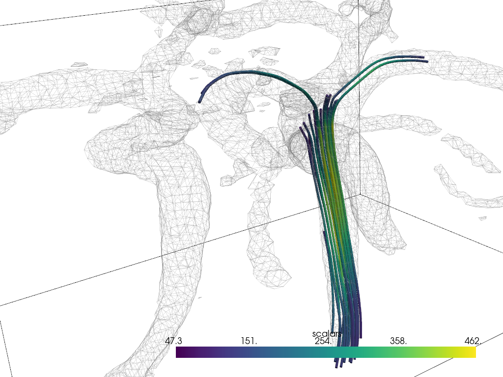
結果を表示します．このデータセットの速度場は低分解能で測定されたため，多くの流線が動脈の外側を通過することに注意してください．

p = pv.Plotter()
p.add_mesh(mesh.outline(), color="k")
p.add_mesh(streamlines.tube(radius=0.15))
p.add_mesh(src)
p.add_mesh(mesh.contour([160]).extract_all_edges(), color="grey", opacity=0.25)
p.camera_position = [(182.0, 177.0, 50), (139, 105, 19), (-0.2, -0.2, 1)]
p.show()

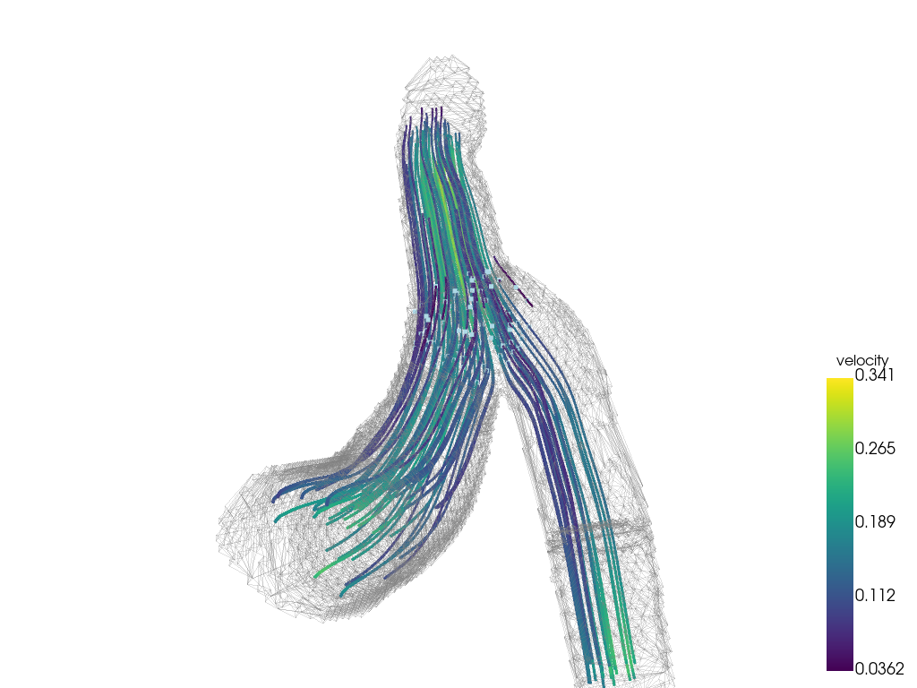
血管

血流の別の例を次に示します:

mesh = examples.download_blood_vessels().cell_data_to_point_data()
mesh.set_active_scalars("velocity")
streamlines, src = mesh.streamlines(
    return_source=True, source_radius=10, source_center=(92.46, 74.37, 135.5)
)

boundary = mesh.decimate_boundary().extract_all_edges()

sargs = dict(vertical=True, title_font_size=16)
p = pv.Plotter()
p.add_mesh(streamlines.tube(radius=0.2), lighting=False, scalar_bar_args=sargs)
p.add_mesh(src)
p.add_mesh(boundary, color="grey", opacity=0.25)
p.camera_position = [(10, 9.5, -43), (87.0, 73.5, 123.0), (-0.5, -0.7, 0.5)]
p.show()

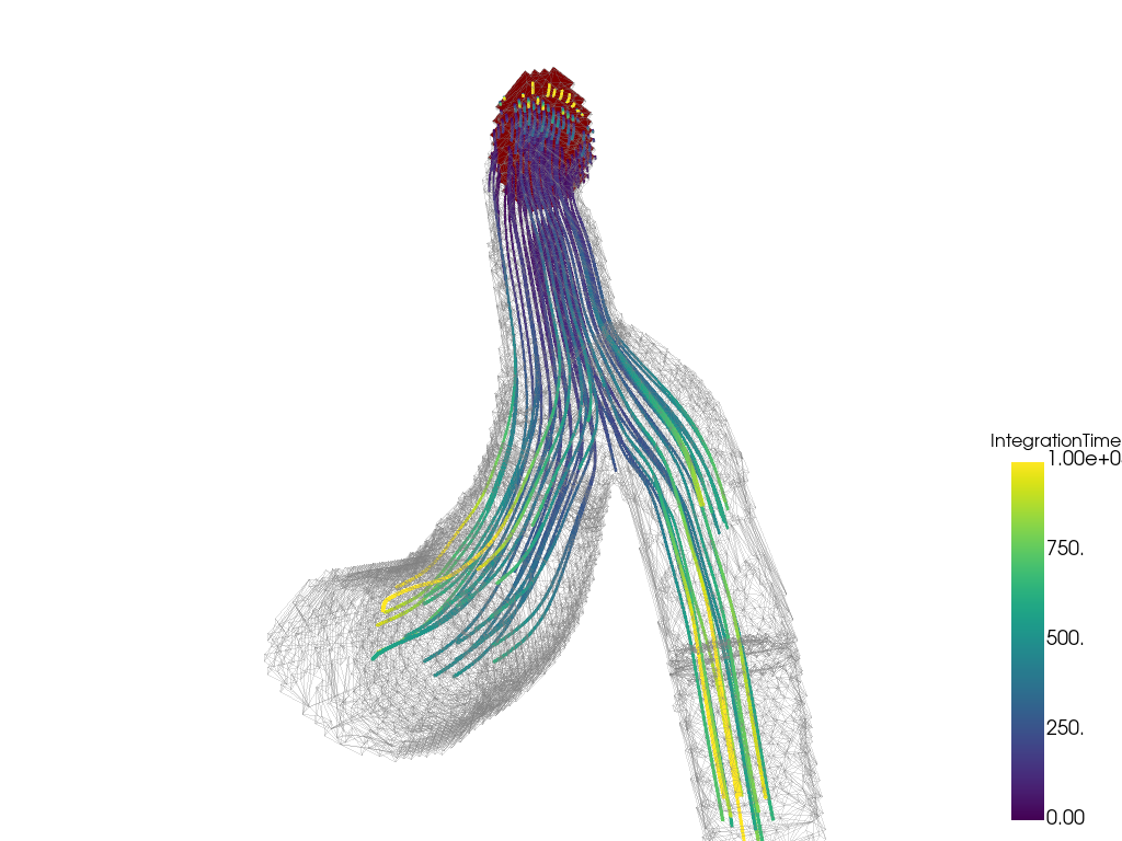
流入口が利用可能な場合などは， pyvista.DataSetFilters.streamlines_from_source() フィルタを使用してソースメッシュを提供することもできます．この例では，流入口を領域のすぐ内側に抽出し，流線の始点として使用します．

source_mesh = mesh.slice('z', origin=(0, 0, 182))  # inlet surface
# thin out ~40% points to get a nice density of streamlines
seed_mesh = source_mesh.decimate_boundary(0.4)
streamlines = mesh.streamlines_from_source(seed_mesh, integration_direction="forward")
# print *only* added arrays from streamlines filter
print("Added arrays from streamlines filter:")
print([array_name for array_name in streamlines.array_names if array_name not in mesh.array_names])

Added arrays from streamlines filter:
['IntegrationTime', 'Vorticity', 'Rotation', 'AngularVelocity', 'Normals', 'ReasonForTermination', 'SeedIds']

時間で着色した流線に沿った流線を流線に沿ってプロットします．

sargs = dict(vertical=True, title_font_size=16)
p = pv.Plotter()
p.add_mesh(
    streamlines.tube(radius=0.2),
    scalars="IntegrationTime",
    clim=[0, 1000],
    lighting=False,
    scalar_bar_args=sargs,
)
p.add_mesh(boundary, color="grey", opacity=0.25)
p.add_mesh(source_mesh, color="red")
p.camera_position = [(10, 9.5, -43), (87.0, 73.5, 123.0), (-0.5, -0.7, 0.5)]
p.show()

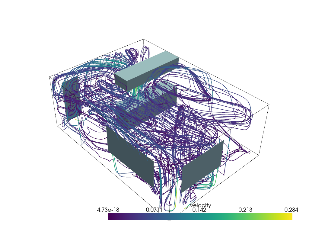
キッチン

kpos = [(-6.68, 11.9, 11.6), (3.5, 2.5, 1.26), (0.45, -0.4, 0.8)]

mesh = examples.download_kitchen()
kitchen = examples.download_kitchen(split=True)

streamlines = mesh.streamlines(n_points=40, source_center=(0.08, 3, 0.71))

p = pv.Plotter()
p.add_mesh(mesh.outline(), color="k")
p.add_mesh(kitchen, color=True)
p.add_mesh(streamlines.tube(radius=0.01), scalars="velocity", lighting=False)
p.camera_position = kpos
p.show()

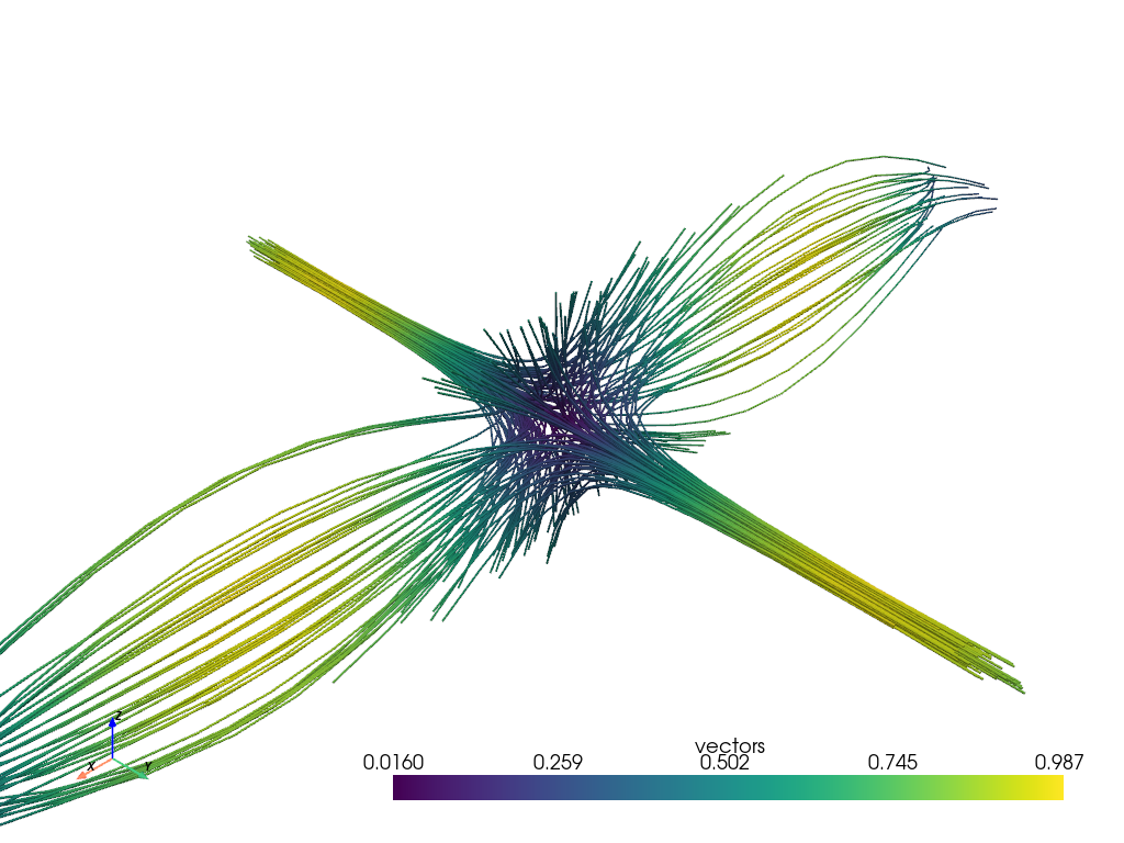
カスタム3 Dベクトルフィールド

nx = 20
ny = 15
nz = 5

origin = (-(nx - 1) * 0.1 / 2, -(ny - 1) * 0.1 / 2, -(nz - 1) * 0.1 / 2)
mesh = pv.ImageData(dimensions=(nx, ny, nz), spacing=(0.1, 0.1, 0.1), origin=origin)
x = mesh.points[:, 0]
y = mesh.points[:, 1]
z = mesh.points[:, 2]
vectors = np.empty((mesh.n_points, 3))
vectors[:, 0] = np.sin(np.pi * x) * np.cos(np.pi * y) * np.cos(np.pi * z)
vectors[:, 1] = -np.cos(np.pi * x) * np.sin(np.pi * y) * np.cos(np.pi * z)
vectors[:, 2] = np.sqrt(3.0 / 3.0) * np.cos(np.pi * x) * np.cos(np.pi * y) * np.sin(np.pi * z)

mesh['vectors'] = vectors

stream, src = mesh.streamlines(
    'vectors', return_source=True, terminal_speed=0.0, n_points=200, source_radius=0.1
)

cpos = [(1.2, 1.2, 1.2), (-0.0, -0.0, -0.0), (0.0, 0.0, 1.0)]
stream.tube(radius=0.0015).plot(cpos=cpos)