pyvista.DataSetFilters.contour

DataSetFilters.contour(

isosurfaces: int | Sequence[float] = 10,

scalars: str | NumpyArray[float] | None = None,

compute_normals: bool = False,

compute_gradients: bool = False,

compute_scalars: bool = True,

rng: VectorLike[float] | None = None,

preference: Literal['point', 'cell'] = 'point',

method: Literal['contour', 'marching_cubes', 'flying_edges'] = 'contour',

progress_bar: bool = False,

)

入力されたコンターを配列で表現します．

isosurfaces はデータ範囲内の等値面の数を指定する整数か，明示的に等値面を設定するための値のシーケンスです．

パラメータ:

isosurfacesint | sequence[float], optional

有効なデータ範囲全体で計算する等値面の数，または等値面として明示的に使用する浮動小数点値のシーケンス．

scalarsstr | array_like[float], optional

閾値を設定するスカラーの名前あるいは配列．これが配列である場合，このフィルタの出力は "Contour Data" として保存されます．デフォルトは，現在アクティブなスカラーです．

compute_normalsbool, default: False

データセットの法線を計算します．

compute_gradientsbool, default: False

データセットの勾配を計算します．

compute_scalarsbool, default: True

輪郭付けされているスカラー値を保持します．

rngsequence[float], optional

等値面の整数が指定されている場合，これは等高線を生成する範囲です．デフォルトはスカラー配列の全データ範囲です．

preferencestr, default: "point"

scalars が指定されている場合，これはデータセット内で検索するために推奨される配列型です． 'point' または 'cell' のいずれかでなければなりません．

methodstr, default: "contour"

コンターの作成に使用するベクトルフィルタを指定します． 'contour' ， 'marching_cubes' および 'flying_edges' のいずれかである必要があります．

progress_barbool, default: False

進行状況を示す進行状況バーを表示します．

戻り値:

pyvista.PolyData

輪郭のある表面．

例

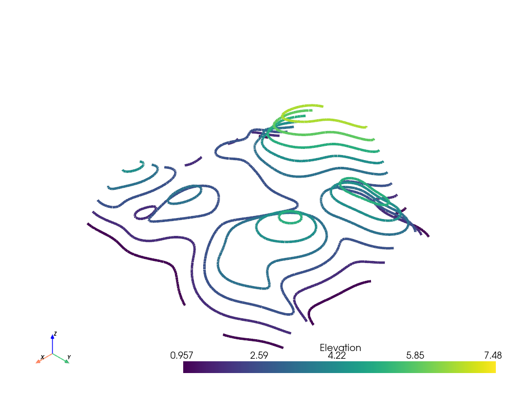
ランダムな丘のデータセットの輪郭を生成します．

>>> from pyvista import examples
>>> hills = examples.load_random_hills()
>>> contours = hills.contour()
>>> contours.plot(line_width=5)

スタティックシーン

インタラクティブなシーン

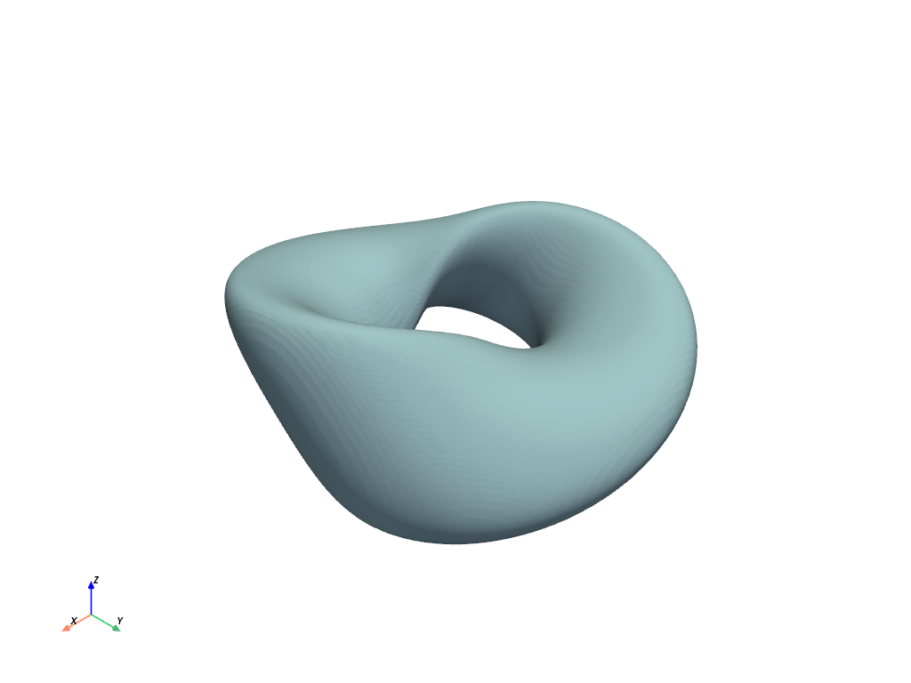
フライングエッジを使ってメビウスの帯の表面を生成します．

>>> import pyvista as pv
>>> a = 0.4
>>> b = 0.1
>>> def f(x, y, z):
...     xx = x * x
...     yy = y * y
...     zz = z * z
...     xyz = x * y * z
...     xx_yy = xx + yy
...     a_xx = a * xx
...     b_yy = b * yy
...     return (
...         (xx_yy + 1) * (a_xx + b_yy)
...         + zz * (b * xx + a * yy)
...         - 2 * (a - b) * xyz
...         - a * b * xx_yy
...     ) ** 2 - 4 * (xx + yy) * (a_xx + b_yy - xyz * (a - b)) ** 2
>>> n = 100
>>> x_min, y_min, z_min = -1.35, -1.7, -0.65
>>> grid = pv.ImageData(
...     dimensions=(n, n, n),
...     spacing=(
...         abs(x_min) / n * 2,
...         abs(y_min) / n * 2,
...         abs(z_min) / n * 2,
...     ),
...     origin=(x_min, y_min, z_min),
... )
>>> x, y, z = grid.points.T
>>> values = f(x, y, z)
>>> out = grid.contour(
...     1,
...     scalars=values,
...     rng=[0, 0],
...     method='flying_edges',
... )
>>> out.plot(color='lightblue', smooth_shading=True)

スタティックシーン

インタラクティブなシーン

このフィルターを使用したその他の例については， 共通フィルタの使用 と マーチングキューブ を参照してください．