電子機器の冷却CFD

SimScale Project Library にあるSimScaleの公開サンプルでホストされているOpenFoamの電子機器冷却CFD例をプロットし， Thermal Management Tutorial: CHT Analysis of an Electronics Box から生成します．

このサンプルデータセットは pyvista.POpenFOAMReader を使って読み込まれ，この README.md に従ってポスト処理されました．

import numpy as np

import pyvista as pv
from pyvista import examples

データセットを読み込む

データセットをダウンロードし，ロードします．

structure データセットは，ファンによって冷却される複数の部品を持つ箱からなり， air データセットは，空気の速度と温度を含むいくつかのスカラー配列を含む空気です．

structure, air = examples.download_electronics_cooling()
structure, air

(PolyData (0x7f218639a7a0)
  N Cells:    344270
  N Points:   187992
  N Strips:   0
  X Bounds:   -3.000e-03, 1.530e-01
  Y Bounds:   -3.000e-03, 2.030e-01
  Z Bounds:   -9.000e-03, 4.200e-02
  N Arrays:   4, UnstructuredGrid (0x7f2186399600)
  N Cells:    1749992
  N Points:   610176
  X Bounds:   -1.388e-18, 1.500e-01
  Y Bounds:   -3.000e-03, 2.030e-01
  Z Bounds:   -6.000e-03, 4.400e-02
  N Arrays:   10)

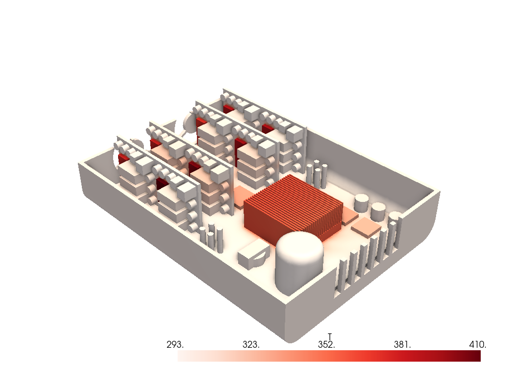
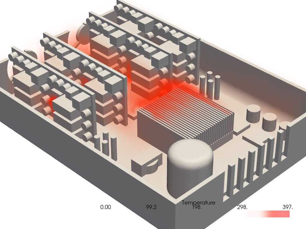
電子機器をプロットする

ここでは， "赤" のカラーマップを使って電子機器の温度をプロットし， enable_ssao() で表面空間の環境オクルージョンを使ってプロットの見た目を改善しました．

pl = pv.Plotter()
pl.enable_ssao(radius=0.01)
pl.add_mesh(
    structure, scalars='T', smooth_shading=True, split_sharp_edges=True, cmap='reds', ambient=0.2
)
pl.enable_anti_aliasing('fxaa')  # also try 'ssaa'
pl.show()

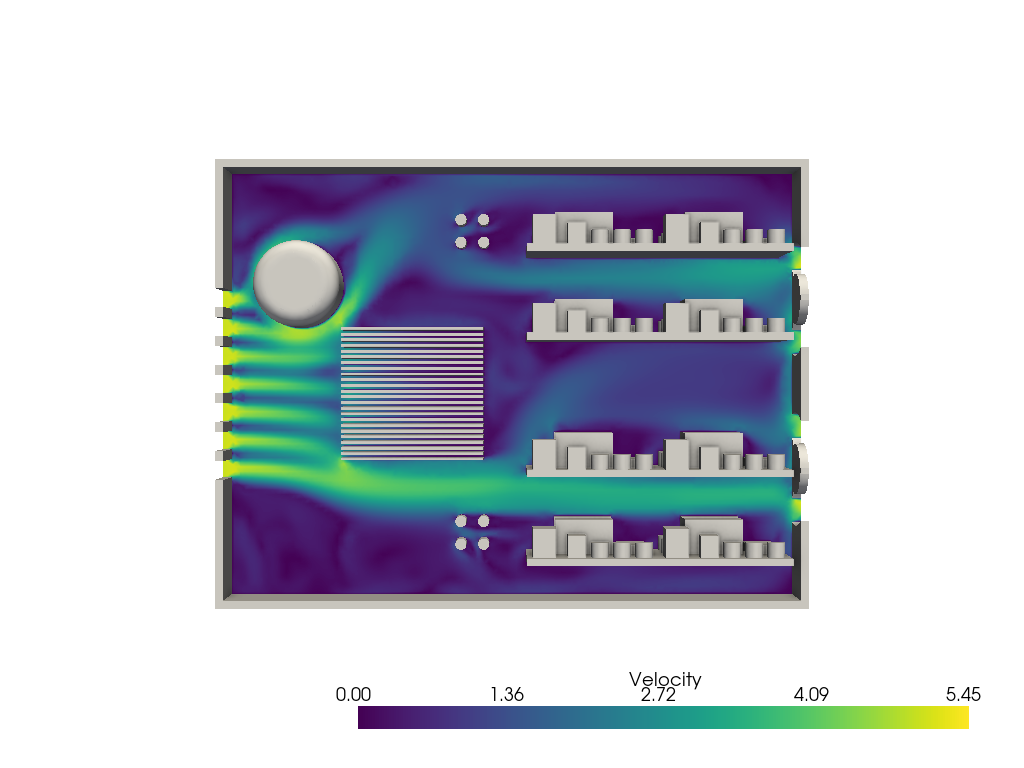
風速のプロット

空気の速度をプロットしてみましょう．

clip() で空気データセットを切り抜き，電子機器と並べてプロットするところから始めます．

ご覧のように，空気はケースの前面(左)から入り，ファンを介してケースの "背面" から押し出されているのです．

# Clip the air in the XY plane
z_slice = air.clip('z', value=-0.005)

# Plot it
pl = pv.Plotter()
pl.enable_ssao(radius=0.01)
pl.add_mesh(z_slice, scalars='U', lighting=False, scalar_bar_args={'title': 'Velocity'})
pl.add_mesh(structure, color='w', smooth_shading=True, split_sharp_edges=True)
pl.camera_position = 'xy'
pl.camera.roll = 90
pl.enable_anti_aliasing('fxaa')
pl.show()

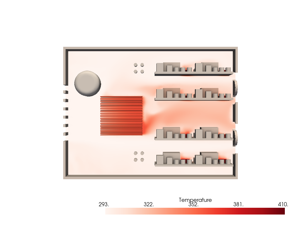
気温のプロット

空気の温度もプロットしてみましょう．今回は，部品の温度もプロットしてみましょう．

pl = pv.Plotter()
pl.enable_ssao(radius=0.01)
pl.add_mesh(
    z_slice, scalars='T', lighting=False, scalar_bar_args={'title': 'Temperature'}, cmap='reds'
)
pl.add_mesh(
    structure,
    scalars='T',
    smooth_shading=True,
    split_sharp_edges=True,
    cmap='reds',
    show_scalar_bar=False,
)
pl.camera_position = 'xy'
pl.camera.roll = 90
pl.enable_anti_aliasing('fxaa')
pl.show()

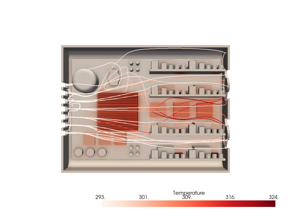
流線のプロット - 流体速度

では，このデータセットの流線をプロットして，空気がケース内をどのように流れているのかを見てみましょう．

streamlines_from_source() を使って流線を生成します．

# Have our streamlines start from the regular openings of the case.
points = []
for x in np.linspace(0.045, 0.105, 7, endpoint=True):
    points.extend([x, 0.2, z] for z in np.linspace(0, 0.03, 5))
points = pv.PointSet(points)
lines = air.streamlines_from_source(points, max_time=2.0)

# Plot
pl = pv.Plotter()
pl.enable_ssao(radius=0.01)
pl.add_mesh(lines, line_width=2, scalars='T', cmap='reds', scalar_bar_args={'title': 'Temperature'})
pl.add_mesh(
    structure,
    scalars='T',
    smooth_shading=True,
    split_sharp_edges=True,
    cmap='reds',
    show_scalar_bar=False,
)
pl.camera_position = 'xy'
pl.camera.roll = 90
pl.enable_anti_aliasing('fxaa')  # also try 'ssaa'
pl.show()

ボリューメトリックプロット - 高温を可視化する

温度の面積の3Dプロットを表示します．

この例では，まず pyvista.UnstructuredGrid から pyvista.ImageData に sample() で結果を抽出してみます．これは add_volume() を使って可視化できるようにするためです．

bounds = np.array(air.bounds) * 1.2
origin = (bounds[0], bounds[2], bounds[4])
spacing = (0.002, 0.002, 0.002)
dimensions = (
    int((bounds[1] - bounds[0]) // spacing[0] + 2),
    int((bounds[3] - bounds[2]) // spacing[1] + 2),
    int((bounds[5] - bounds[4]) // spacing[2] + 2),
)
grid = pv.ImageData(dimensions=dimensions, spacing=spacing, origin=origin)
grid = grid.sample(air)

opac = np.zeros(20)
opac[1:] = np.geomspace(1e-7, 0.1, 19)
opac[-5:] = [0.05, 0.1, 0.5, 0.5, 0.5]

pl = pv.Plotter()
pl.add_mesh(structure, color='w', smooth_shading=True, split_sharp_edges=True)
vol = pl.add_volume(
    grid,
    scalars='T',
    opacity=opac,
    cmap='autumn_r',
    show_scalar_bar=True,
    scalar_bar_args={'title': 'Temperature'},
)
vol.prop.interpolation_type = 'linear'
pl.camera.zoom(2)
pl.show()