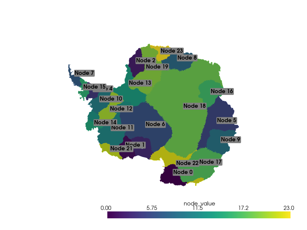
メッシュ領域間でフィールドを比較

氷河モデリングシミュレーションの速度データをシミュレーションのノード間で比較したものです．メッシュを簡略化して，シミュレーションノードの値がすでにメッシュ上にあるようにしました．

これは元々 pyvista/pyvista-support#83 に投稿されました．

モデリング結果は`Urruty Benoit <BenoitURRUTY>`_ の好意により Elmer/Ice シミュレーションソフトウェアから得たものである．

import numpy as np

import pyvista as pv
from pyvista import examples

# Load the sample data
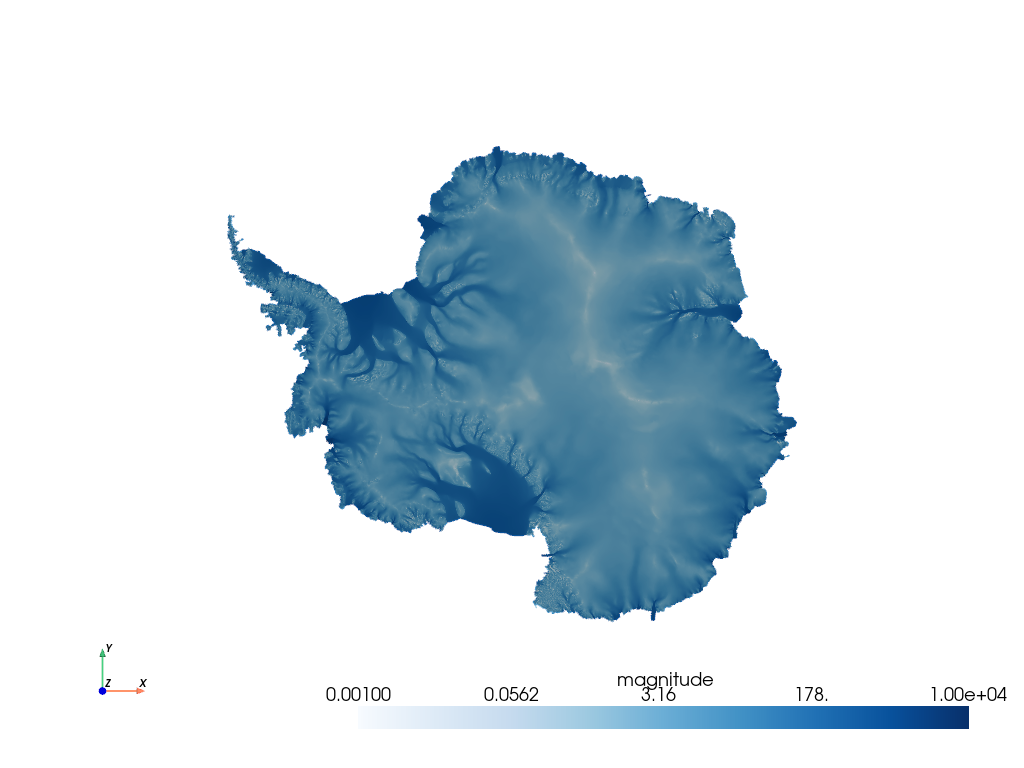
mesh = examples.download_antarctica_velocity()
mesh["magnitude"] = np.linalg.norm(mesh["ssavelocity"], axis=1)
mesh

Header	Data Arrays
PolyData Information N Cells 1106948 N Points 557470 N Strips 0 X Bounds -2.506e+06, 2.743e+06 Y Bounds -2.143e+06, 2.240e+06 Z Bounds 0.000e+00, 0.000e+00 N Arrays 3	Name Field Type N Comp Min Max ssavelocity Points float64 3 -4.341e+03 9.677e+03 node_value Points int64 1 0.000e+00 2.300e+01 magnitude Points float64 1 6.649e-03 1.013e+04

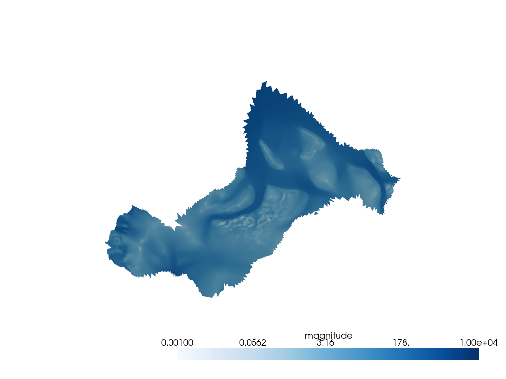
ここには，シミュレーションノードに基づいてメッシュの領域を抽出するヘルパーがあります．

def extract_node(node):
    idx = mesh["node_value"] == node
    return mesh.extract_points(idx)

p = pv.Plotter()
p.add_mesh(mesh, scalars="node_value")
for node in np.unique(mesh["node_value"]):
    loc = extract_node(node).center
    p.add_point_labels(loc, [f"Node {node}"])
p.show(cpos="xy")

vel_dargs = dict(scalars="magnitude", clim=[1e-3, 1e4], cmap='Blues', log_scale=True)

mesh.plot(cpos="xy", **vel_dargs)

a = extract_node(12)
b = extract_node(20)

pl = pv.Plotter()
pl.add_mesh(a, **vel_dargs)
pl.add_mesh(b, **vel_dargs)
pl.show(cpos='xy')

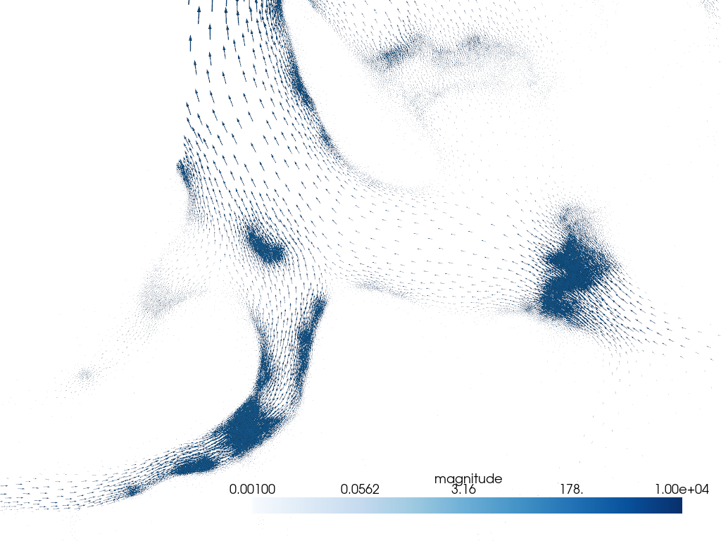
メッシュなしでベクトルをプロット

pl = pv.Plotter()
pl.add_mesh(a.glyph(orient="ssavelocity", factor=20), **vel_dargs)
pl.add_mesh(b.glyph(orient="ssavelocity", factor=20), **vel_dargs)
pl.camera_position = [
    (-1114684.6969340036, 293863.65389149904, 752186.603224546),
    (-1114684.6969340036, 293863.65389149904, 0.0),
    (0.0, 1.0, 0.0),
]
pl.show()

方向を比較します．適切な方向比較ができるように正規化します．

flow_a = a.point_data['ssavelocity'].copy()
flow_a /= np.linalg.norm(flow_a, axis=1).reshape(-1, 1)
flow_b = b.point_data['ssavelocity'].copy()
flow_b /= np.linalg.norm(flow_b, axis=1).reshape(-1, 1)


# plot normalized vectors
pl = pv.Plotter()
pl.add_arrows(a.points, flow_a, mag=10000, color='b', label='flow_a')
pl.add_arrows(b.points, flow_b, mag=10000, color='r', label='flow_b')
pl.add_legend()
pl.camera_position = [
    (-1044239.3240694795, 354805.0268606294, 484178.24825854995),
    (-1044239.3240694795, 354805.0268606294, 0.0),
    (0.0, 1.0, 0.0),
]
pl.show()

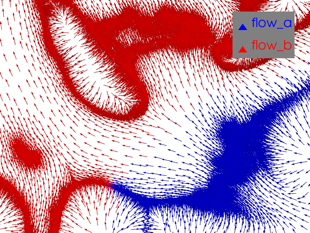
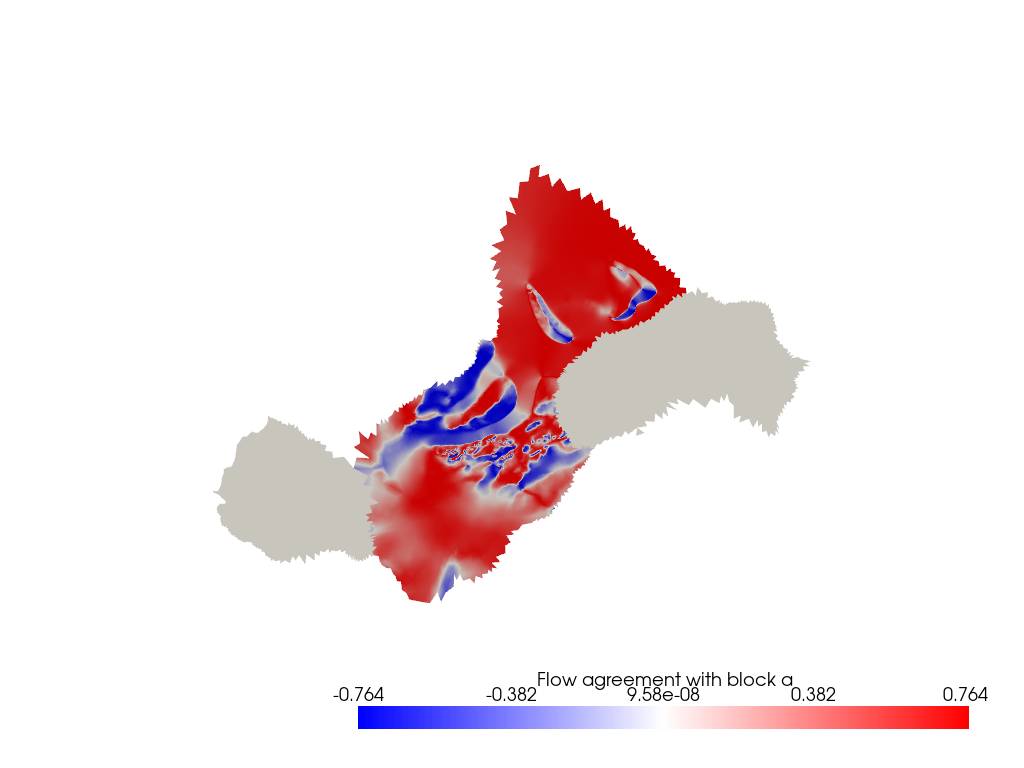
flow_b の平均流路と一致する flow_a

agree = flow_a.dot(flow_b.mean(0))

pl = pv.Plotter()
pl.add_mesh(a, scalars=agree, cmap='bwr', scalar_bar_args={'title': 'Flow agreement with block b'})
pl.add_mesh(b, color='w')
pl.show(cpos='xy')

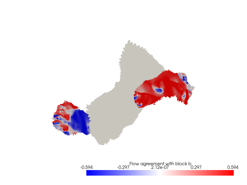
agree = flow_b.dot(flow_a.mean(0))

pl = pv.Plotter()
pl.add_mesh(a, color='w')
pl.add_mesh(b, scalars=agree, cmap='bwr', scalar_bar_args={'title': 'Flow agreement with block a'})
pl.show(cpos='xy')