表面の法線を計算します

表面上の法線を計算します．

import numpy as np

from pyvista import examples

mesh = examples.download_topo_global()
mesh.plot(cmap="gist_earth", show_scalar_bar=False)

スタティックなシーン

インタラクティブなシーン

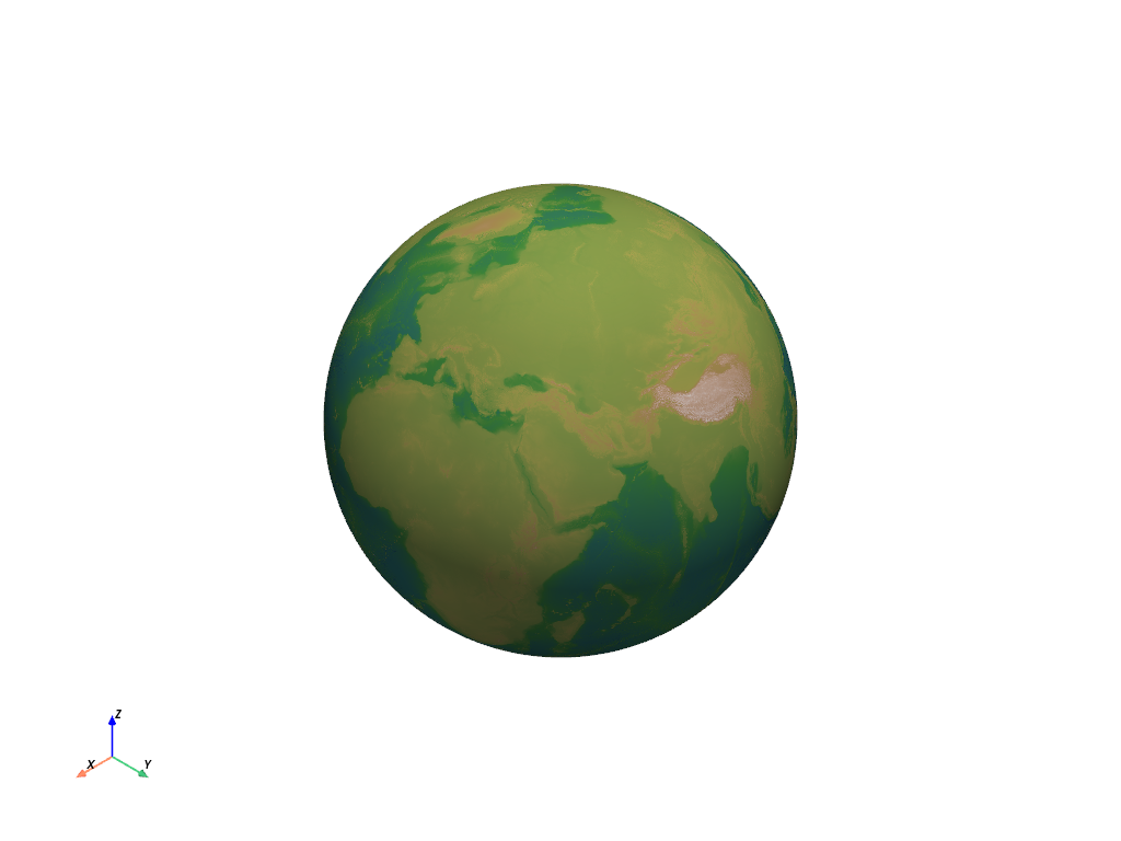
これで地球のサーフェスデータセットがロードされました．残念ながら，データセットには地形起伏を隠す均一な半径の地球が表示されます． pyvista.PolyData.compute_normals() を使用して，データセット内のすべてのポイントで地球上の法線ベクトルを計算し，データセットで指定された値を使用してサーフェスを法線方向にワープし，誇張された地形レリーフを作成します．

# Compute the normals in-place and use them to warp the globe
mesh.compute_normals(inplace=True)  # this activates the normals as well

Header	Data Arrays
PolyData Information N Cells 2333880 N Points 2336041 N Strips 0 X Bounds -1.000e+00, 1.000e+00 Y Bounds -1.000e+00, 1.000e+00 Z Bounds -1.000e+00, 1.000e+00 N Arrays 3	Name Field Type N Comp Min Max altitude Points float32 1 -1.042e+04 6.527e+03 Normals Points float32 3 -1.000e+00 1.000e+00 Normals Cells float32 3 -1.000e+00 1.000e+00

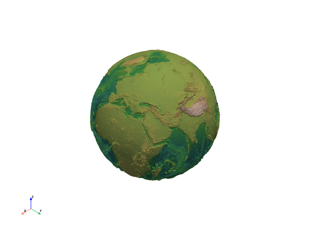
次に，これらの法線を使用して，サーフェスをワープさせます．

warp = mesh.warp_by_scalar(factor=0.5e-5)

そして，見てみよう!

warp.plot(cmap="gist_earth", show_scalar_bar=False)

スタティックなシーン

インタラクティブなシーン

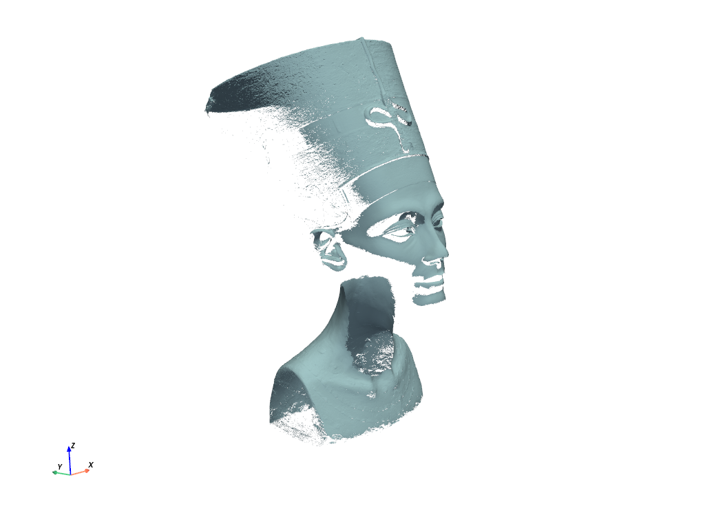
面またはセル法線を使用して，一般的な方向を向いているメッシュのすべての面を抽出することもできます．次のスニペットでは，メッシュを取得し，そのセル面に沿って法線を計算し，上向きの面を抽出します．

mesh = examples.download_nefertiti()
# Compute normals
mesh.compute_normals(cell_normals=True, point_normals=False, inplace=True)

# Get list of cell IDs that meet condition
ids = np.arange(mesh.n_cells)[mesh["Normals"][:, 2] > 0.0]

# Extract those cells
top = mesh.extract_cells(ids)

cpos = [
    (-834.3184529757553, -918.4677714398535, 236.5468795300025),
    (11.03829376004883, -13.642289291587957, -35.91218884207208),
    (0.19212361465657216, 0.11401076390090074, 0.9747256344254143),
]

top.plot(cpos=cpos, color=True)

スタティックなシーン

インタラクティブなシーン