注釈
完全なサンプルコードをダウンロードしたり、Binderを使ってブラウザでこのサンプルを実行するには、 最後に進んでください 。
レッスンの概要#
この演習では,最初のレッスンの例の概要を説明しますので,試してみてください!
import numpy as np
import pyvista as pv
from pyvista import examples
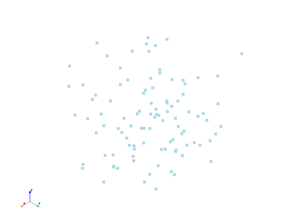
ポイントとは?#
ポイントクラウドから始めましょう - これは頂点のみを持つメッシュタイプです.作成するには,2 D配列の直交座標を次のように定義します.
points = np.random.rand(100, 3)
points[:5, :]  # output first 5 rows
array([[0.01893663, 0.93874832, 0.03705064],
       [0.73259084, 0.95062743, 0.8254343 ],
       [0.82264789, 0.56134719, 0.44609905],
       [0.12163566, 0.55151668, 0.80501852],
       [0.4893341 , 0.32402678, 0.84573917]])
点 (n x 3) の numpy 配列を PolyData に渡します.
mesh.plot(point_size=10, style="points")
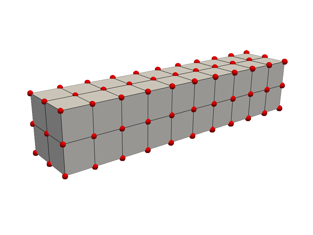
しかし,ほとんどのメッシュは,この格子状のメッシュのように,点と点の間に何らかのつながりがあることに注意が必要です.
mesh = examples.load_hexbeam()
cpos = [(6.20, 3.00, 7.50), (0.16, 0.13, 2.65), (-0.28, 0.94, -0.21)]

pl = pv.Plotter()
pl.add_mesh(mesh, show_edges=True, color="white")
pl.add_points(mesh.points, color="red", point_size=20, render_points_as_spheres=True)
pl.camera_position = cpos
pl.show()
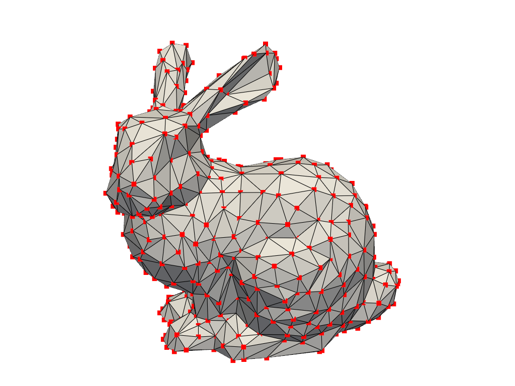
mesh = examples.download_bunny_coarse()

pl = pv.Plotter()
pl.add_mesh(mesh, show_edges=True, color="white")
pl.add_points(mesh.points, color="red", point_size=10)
pl.camera_position = [(0.02, 0.30, 0.73), (0.02, 0.03, -0.022), (-0.03, 0.94, -0.34)]
pl.show()
セルとは?#
セルとは,メッシュの接続性またはトポロジーを定義する点間のジオメトリです.上記の例では,セルは線(黒で着色されたエッジ)と接続点(赤で着色された)によって定義されています.例えば,ビームの例におけるセルは,そのメッシュの8つの点の間の領域によって定義されるボクセルである.ここでは,メッシュから1つのセルを取り出し,その情報を表示し,メッシュの中での位置をプロットすることができます.
mesh = examples.load_hexbeam()

single_cell = mesh.get_cell(mesh.n_cells - 1)
single_cell
Cell (0x7fc59bed0580)
  Type:        <CellType.HEXAHEDRON: 12>
  Linear:      True
  Dimension:   3
  N Points:    8
  N Faces:     6
  N Edges:     12
  X Bounds:    5.000e-01, 1.000e+00
  Y Bounds:    5.000e-01, 1.000e+00
  Z Bounds:    4.500e+00, 5.000e+00
pl = pv.Plotter()
pl.add_mesh(mesh, show_edges=True, color="white")
pl.add_points(mesh.points, color="red", point_size=20)
pl.add_mesh(
    single_cell.cast_to_unstructured_grid(),
    color="pink",
    edge_color="blue",
    line_width=5,
    show_edges=True,
)
pl.camera_position = [(6.20, 3.00, 7.50), (0.16, 0.13, 2.65), (-0.28, 0.94, -0.21)]
pl.show()
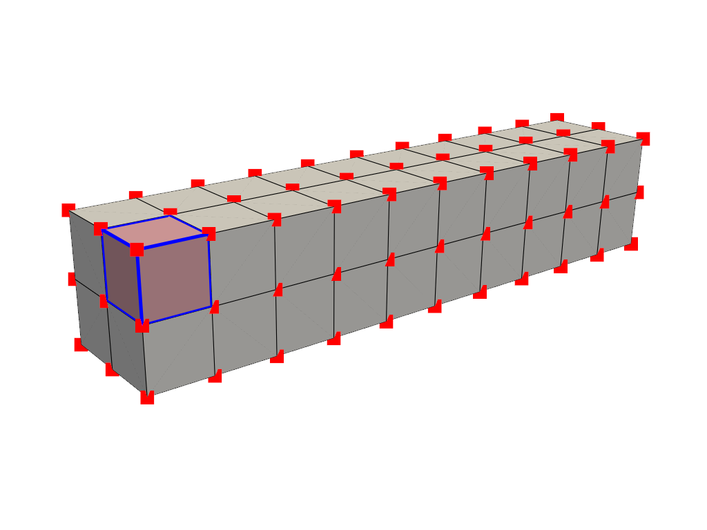
セルはボクセルに限らず,3点間の三角形や2点間の線,あるいは1点をセルとすることもできます(ただし,これは特殊なケースです).
アトリビュートとは?#
アトリビュートは,メッシュのポイントまたはセルに存在するデータ値です.PyVistaでは,ポイントデータとセルデータの両方を処理し,データ辞書に簡単にアクセスして,メッシュのすべてのポイントまたはすべてのセルに存在するアトリビュートの配列を保持できます.これらの属性は,以下のようにアクセスできるPyVistaメッシュに付けられた辞書のような属性にアクセスできます.
ポイントデータ#
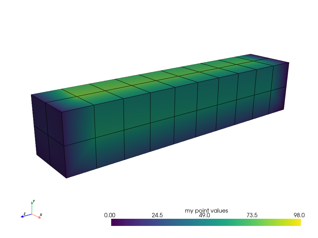
点データとは,メッシュの各点に存在する値(スカラー,ベクトルなど)の配列のことです.属性配列の各要素は,メッシュの各点に対応します.梁のメッシュの点データを作ってみましょう.プロットする場合,点間の値はセルをまたいで補間されます.
mesh.point_data["my point values"] = np.arange(mesh.n_points)
mesh.plot(scalars="my point values", cpos=cpos, show_edges=True)
セルデータ#
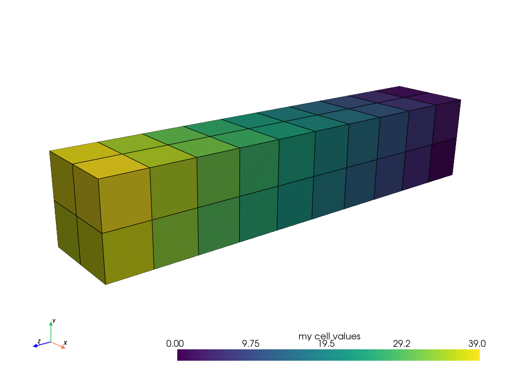
セルデータは,メッシュの各セル全体に存在する値の配列(スカラー,ベクトルなど)を参照します.つまり,セル全体(2 D面または3 D体積)にそのアトリビュートの値が割り当てられます.
mesh.cell_data["my cell values"] = np.arange(mesh.n_cells)
mesh.plot(scalars="my cell values", cpos=cpos, show_edges=True)
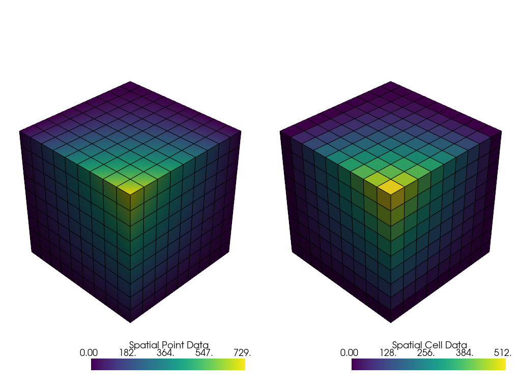
ここでは,点データとセルデータを比較し,色をマッピングするときに点データがセル間でどのように補間されるかを示します.これは,セルのドメイン全体で単一の値を持つセルデータとは異なります.
import pyvista as pv
from pyvista import examples

uni = examples.load_uniform()

pl = pv.Plotter(shape=(1, 2), border=False)
pl.add_mesh(uni, scalars="Spatial Point Data", show_edges=True)
pl.subplot(0, 1)
pl.add_mesh(uni, scalars="Spatial Cell Data", show_edges=True)
pl.link_views()
pl.show()
フィールドデータ#
フィールドデータはポイントやセルとは直接関連していませんが,メッシュに添付する必要があります. これはメモを格納した文字列の配列であったりします.
mesh = pv.Cube()
mesh.field_data["metadata"] = ["Foo", "bar"]
mesh.field_data
pyvista DataSetAttributes
Association     : NONE
Contains arrays :
    metadata                <U3        (2,)
スカラーをメッシュに割り当てる#
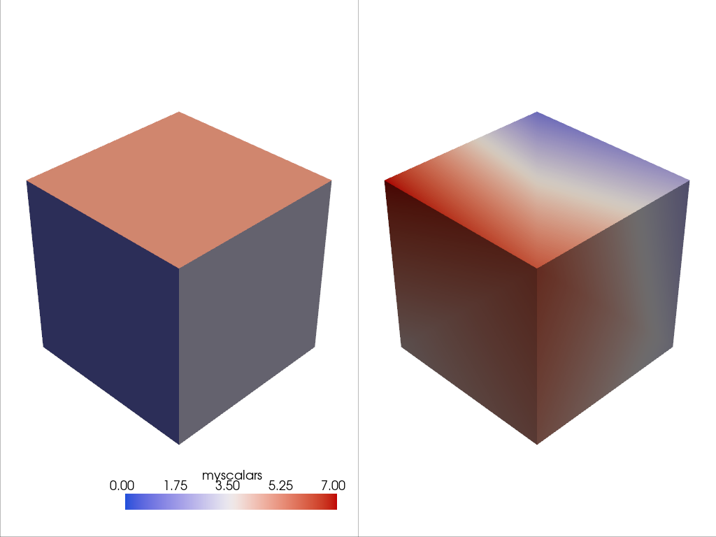
ここでは,セルの属性に値を割り当て,それをプロットする方法を紹介します. ここでは,6つの面を含む立方体を生成し,それぞれの面に range(6) から整数を割り当てて,それをプロットしています.
これは,各点にスカラーを割り当てるのとは異なることに注意してください.
cube = pv.Cube()
cube.cell_data["myscalars"] = range(6)

other_cube = cube.copy()
other_cube.point_data["myscalars"] = range(8)

pl = pv.Plotter(shape=(1, 2), border_width=1)
pl.add_mesh(cube, cmap="coolwarm")
pl.subplot(0, 1)
pl.add_mesh(other_cube, cmap="coolwarm")
pl.show()
Total running time of the script: (0 minutes 3.318 seconds)